Introduction

Artificial Intelligence has been witnessing a monumental growth in bridging the gap between the capabilities of humans and machines. Researchers and enthusiasts alike, work on numerous aspects of the field to make amazing things happen. One of many such areas is the domain of Computer Vision.

The agenda for this field is to enable machines to view the world as humans do, perceive it in a similar manner, and even use the knowledge for a multitude of tasks such as Image & Video recognition, Image Analysis & Classification, Media Recreation, Recommendation Systems, Natural Language Processing, etc. The advancements in Computer Vision with Deep Learning has been constructed and perfected with time, primarily over one particular algorithm — a Convolutional Neural Network (CNN, ConvNet).

Let’s first discuss the difference between Object detection algorithms and Classification algorithms:

Object detection aids in pose estimation, vehicle detection, surveillance, etc. The difference between object detection algorithms and classification algorithms is that in detection algorithms, we try to draw a bounding box around the object of interest to locate it within the image. Also, you might not necessarily draw just one bounding box in an object detection case, there could be many bounding boxes representing different objects of interest within the image and you would not know how many beforehand.

Types of CNN (Convolution Neural Network) we will discuss:

1. Standard CNN
2. R-CNN
3. Fast-CNN
4. Faster-R-CNN

Standard CNN

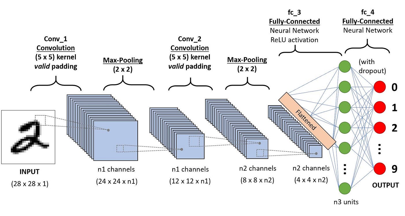
A convolutional neural network consists of an input layer, hidden layers, and an output layer. In any feed-forward neural network, any middle layers are called hidden because their inputs and outputs are masked by the activation function and final convolution. In a convolutional neural network, the hidden layers include layers that perform convolutions. Typically this includes a layer that performs a dot product of the convolution kernel with the layer’s input matrix. This product is usually the Frobenius inner product, and its activation function is commonly ReLU. As the convolution kernel slides along the input matrix for the layer, the convolution operation generates a feature map, which in turn contributes to the input of the next layer. This is followed by other layers such as pooling layers, fully connected layers, and normalization layers.

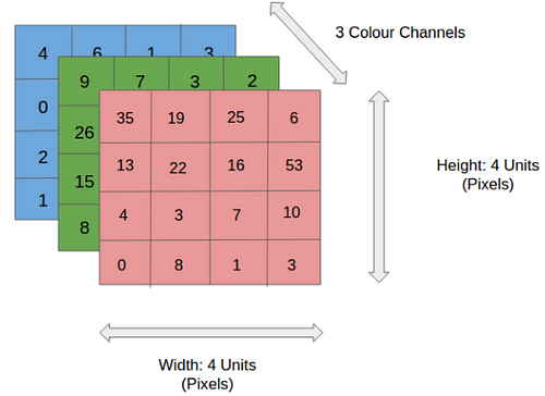
Input Image

Convolution Layer — The Kernel

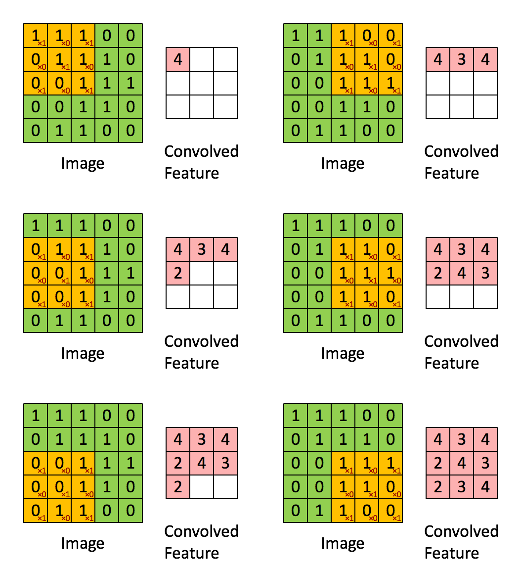
The role of the Convolution layers is to reduce the images into a form that is easier to process, without losing features that are critical for getting a good prediction. This is important when we are to design an architecture that is not only good at learning features but also is scalable to massive datasets.

Pooling Layer

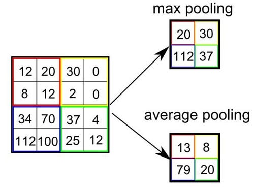
Similar to the Convolutional Layer, the Pooling layer is responsible for reducing the spatial size of the Convolved Feature. This is to decrease the computational power required to process the data through dimensionality reduction. Furthermore, it is useful for extracting dominant features which are rotational and positional invariant, thus maintaining the process of effectively training the model.

There are two types of Pooling: Max Pooling and Average Pooling. Max Pooling returns the maximum value from the portion of the image covered by the Kernel. On the other hand, Average Pooling returns the average of all the values from the portion of the image covered by the Kernel.

Classification — Fully Connected Layer (FC Layer)

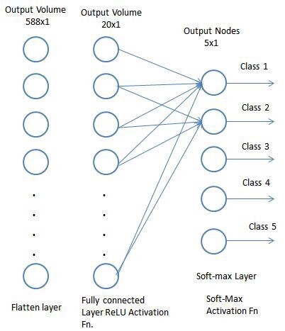
Adding a Fully-Connected layer is a (usually) cheap way of learning non-linear combinations of the high-level features as represented by the output of the convolutional layer. The Fully-Connected layer is learning a possibly non-linear function in that space.

R-CNN

To bypass the problem of selecting a huge number of regions, Ross Girshick et al. proposed a method where we use selective search to extract just 2000 regions from the image and he called them region proposals. Therefore, now, instead of trying to classify a huge number of regions, you can just work with 2000 regions. These 2000 region proposals are generated using the selective search algorithm which is written below.

Steps

1. Generate initial sub-segmentation, we generate many candidates regions
2. Use greedy algorithm to recursively combine similar regions into larger ones
3. Use the generated regions to produce the final candidate region proposals

To know more about the Selective Search Algorithm, follow this link. These 2000 candidate region proposals are warped into a square and fed into a Convolutional Neural Network that produces a 4096-dimensional feature vector as output. The CNN acts as a feature extractor and the output dense layer consists of the features extracted from the image and the extracted features are fed into an SVM to classify the presence of the object within that candidate region proposal. In addition to predicting the presence of an object within the region proposals, the algorithm also predicts four values which are offset values to increase the precision of the bounding box. For example, given a region proposal, the algorithm would have predicted the presence of a person but the face of that person within that region proposal could’ve been cut in half. Therefore, the offset values help in adjusting the bounding box of the region proposal.

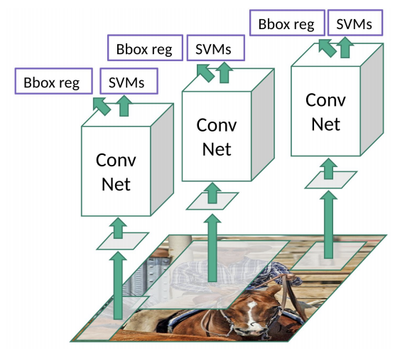
Problems with R-CNN

1. It still takes a huge amount of time to train the network as you would have to classify 2000 region proposals per image.
2. It cannot be implemented real time as it takes around 47 seconds for each test image.
3. The selective search algorithm is a fixed algorithm. Therefore, no learning is happening at that stage. This could lead to the generation of bad candidate region proposals.

Fast R-CNN

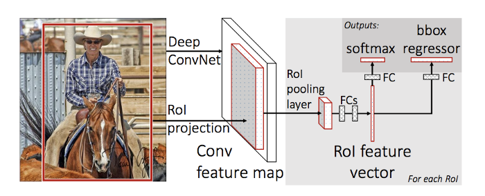
The same author of the previous paper(R-CNN) solved some of the drawbacks of R-CNN to build a faster object detection algorithm and it was called Fast R-CNN. The approach is similar to the R-CNN algorithm. But, instead of feeding the region proposals to the CNN, we feed the input image to the CNN to generate a convolutional feature map. From the convolutional feature map, we identify the region of proposals and warp them into squares and by using an ROI pooling layer we reshape them into a fixed size so that it can be fed into a fully connected layer. From the RoI feature vector, we use a softmax layer to predict the class of the proposed region and the offset values for the bounding box.

The reason “Fast R-CNN” is faster than R-CNN is because you don’t have to feed 2000 region proposals to the Convolutional Neural Network every time. Instead, the convolution operation is done only once per image and a feature map is generated from it.

ROI Pooling Layer

Faster R-CNN

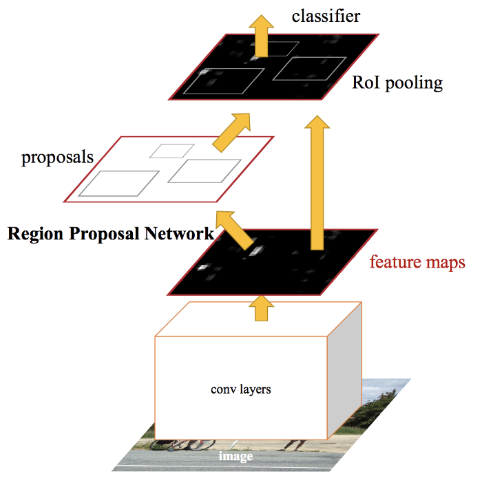
Both of the above algorithms (R-CNN & Fast R-CNN) uses selective search to find out the region proposals. Selective search is a slow and time-consuming process affecting the performance of the network. Therefore, Shaoqing Ren et al. came up with an object detection algorithm that eliminates the selective search algorithm and lets the network learn the region proposals.

Similar to Fast R-CNN, the image is provided as an input to a convolutional network which provides a convolutional feature map. Instead of using a selective search algorithm on the feature map to identify the region proposals, a separate network is used to predict the region proposals. The predicted region proposals are then reshaped using an ROI pooling layer which is then used to classify the image within the proposed region and predict the offset values for the bounding boxes.

Conclusion

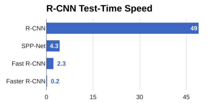
From the above graph, you can see that Faster R-CNN is much faster than its predecessors. Therefore, it can even be used for real-time object detection.

References

1. https://en.wikipedia.org/wiki/Convolutional_neural_network
2. https://towardsdatascience.com/r-cnn-fast-r-cnn-faster-r-cnn-yolo-object-detection-algorithms-36d53571365e